


Reporting confidence intervals in scientific articles is important and relevant for evidence-based practice. Clinicians should understand confidence intervals in order to determine if they can realistically expect results similar to those presented in research studies when they implement the scientific evidence in clinical practice. The aims of this masterclass are: (1) to discuss confidence intervals around effect estimates; (2) to understand confidence intervals estimation (frequentist and Bayesian approaches); and (3) to interpret such uncertainty measures.
ContentConfidence intervals are measures of uncertainty around effect estimates. Interpretation of the frequentist 95% confidence interval: we can be 95% confident that the true (unknown) estimate would lie within the lower and upper limits of the interval, based on hypothesized repeats of the experiment. Many researchers and health professionals oversimplify the interpretation of the frequentist 95% confidence interval by dichotomizing it in statistically significant or non-statistically significant, hampering a proper discussion on the values, the width (precision) and the practical implications of such interval. Interpretation of the Bayesian 95% confidence interval (which is known as credible interval): there is a 95% probability that the true (unknown) estimate would lie within the interval, given the evidence provided by the observed data.
ConclusionsThe use and reporting of confidence intervals should be encouraged in all scientific articles. Clinicians should consider using the interpretation, relevance and applicability of confidence intervals in real-world decision-making. Training and education may enhance knowledge and skills related to estimating, understanding and interpreting uncertainty measures, reducing the barriers for their use under either frequentist or Bayesian approaches.
A paper published within this issue of the Brazilian Journal of Physical Therapy (BJPT) raised a very interesting, important and relevant matter for evidence-based practice: the use of the 95% confidence interval (CI) for reporting the uncertainty around between-group comparisons in randomized controlled trials investigating the effects of physical therapy interventions.1 Briefly, the study found that: (1) only less than one-third of physical therapy trials report CIs; (2) trials with lower risk of bias (i.e., higher quality) are more likely to report CIs; and (3) there has been a consistent increase in reporting CIs over time.1 The increasing trend on reporting CIs is good news for physical therapy evidence-based practice. Nevertheless, clinicians should understand CIs so they can appropriately interpret results of trials in order to better implement such evidence in practice. Therefore, this masterclass is aimed at: (1) discussing CIs around effect estimates on continuous (mean and mean difference) and dichotomous (proportion, odds, absolute risk reduction [ARR], relative risk [RR] and odds ratio [OR]) outcomes; (2) understanding CIs estimation (frequentist and Bayesian approaches); and (3) interpreting such uncertainty measures. We believe that this initiative might help clinicians to achieve the purpose of better understanding and interpreting uncertainty measures around effect estimates.
What are confidence intervals?A CI is a measure of the uncertainty around the effect estimate. It is an interval composed of a lower and an upper limit, which indicates that the true (unknown) effect may be somewhere within this interval. The effect presented in the scientific report must always be inside the CI reported, and the width of the interval represents the precision of the effect estimate. Therefore, the narrower the CI the more precise is the effect estimate. The CI width (degree of uncertainty) varies according to two factors: (1) sample size (n); and (2) heterogeneity (standard deviation [SD] or standard error [SE]) contained in the study. The sample size is inversely proportional to the degree of uncertainty; the larger the sample size, the smaller the CI width, which would indicate a lower degree of uncertainty. However, heterogeneity is directly proportional to the degree of uncertainty; the lower the heterogeneity the lower the uncertainty. This means that studies presenting lower SDs or SEs have a lower degree of uncertainty and a narrower CI.
The confidence (probability) level (i.e., 95%) of the CI represents the accuracy of the effect estimate.2 For example, the 99% CI is more accurate than the 95% CI, because it captures a broader spectrum of the data distribution. Thereby, the 99% CI is wider than the 95% CI. However, the trade-off is that the 99% CI is less precise than the 95% CI. The decision of using a certain confidence level should consider a balance between accuracy and precision. In health sciences the 95% confidence level is most often used. Two common approaches to estimate CIs are the frequentist and the Bayesian. In the next sections we will discuss the following topics related to both approaches: how to estimate; how to interpret; advantages; disadvantages; and illustrative examples (with case studies described in Boxes 1 and 2).
Case study of a randomized controlled trial (RCT) with a continuous outcome.
Parreira et al.21 have conducted a RCT aimed at investigating the effects of Kinesio Taping applied according to the manuals (nI=74) compared to sham applications (nC=74) in individuals with chronic nonspecific low back pain. One of the primary outcomes was pain intensity measured with a numeric pain rating scale (NPRS) ranging from 0 (no pain) to 10 (worst possible pain). The table below describes the results for each group at baseline and after four weeks from baseline.
| Intervention group Mean (SD) | Comparison group Mean (SD) | Mean between-group diff (95% CI) | |
|---|---|---|---|
| Baseline | 7.0 (2.0) | 6.8 (2.0) | 0.2 (−0.4 to 0.8) |
| 4 weeks | 4.4 (2.8) | 4.6 (2.5) | −0.2 (−1.1 to 0.7) |
| Within-group diff | −2.6 (3.1) | −2.2 (2.7) | −0.4 (−1.3 to 0.5) |
SD, standard deviation. CI, frequentist confidence interval. “diff”, difference.
Mean difference between groups
The recommended outcome of RCTs investigating continuous variables, as the NPRS, is the between-group difference of the within-group difference. This outcome is usually obtained from the regression coefficient representing the interaction term composed of group and time in linear mixed models.22 Simplifying, the interaction term can also be estimated using a table like the one above. Therefore, the effect found for pain intensity after four weeks from baseline in this study was −0.4, which means that the intervention group reduced 0.4 more points in the 11-point NPRS compared to the control group.
95% confidence interval (CI)
- Standard error (SE): Eq. (2.1)
• SEdiff=√(((nI−1)SDI2)+((nC−1)SDC2)/(nI+nC−2))×√((1/nI)+(1/nC))
• SEdiff=√((((74−1)3.12)+((74−1)2.72))/(74+74−2))×√((1/74)+(1/74))=0.478
- t(probability=0.95; df=74+74−2)=1.976346≈1.96
- 95% CI=(meanI−meanC)±(t×SEdiff)=(−2.6−(−2.2))±(1.96×0.478)=−1.3 to 0.5
The 95% frequentist CI around the effect found for pain intensity after four weeks from baseline in the study of Parreira et al.21 was −1.3 to 0.5 in the 11-point NPRS. This means that we can be 95% confident that individuals with chronic nonspecific low back pain would present, on average, a mean difference between −1.3 and 0.5 when comparing the intervention with the comparison group, based on hypothesized repeats of the experiment. Since the 95% CI contains the null effect (i.e., zero), which represents the null hypothesis (i.e., no difference between the groups), we cannot be 95% confident that the intervention group would present a reduced pain intensity compared to the comparison group in repeats of the experiment, as suggested by the effect estimate (i.e., −0.4). Therefore, we can conclude that this effect was not statically significant, which means that this evidence supports the null hypothesis. In other words, there was no difference between the groups.
Case study of a randomized controlled trial (RCT) with a dichotomous outcome.
Mateus-Vasconcelos et al.23 have conducted a RCT aimed at investigating the effects of vaginal palpation, vaginal palpation associated with posterior pelvic tilt, and intravaginal electrical stimulation in facilitating voluntary contraction of the pelvic floor muscles in women with pelvic floor dysfunctions. This case study is considering only the vaginal palpation associated with posterior pelvic tilt as the intervention group (nI=33), and verbal instructions to perform pelvic floor muscle exercises at home as the comparison group (nC=33). The primary outcomes was the number of women who had changed in the Modified Oxford Scale (MOS) for pelvic floor muscle strength, ranging from 0 (no contraction) to 5 (strong contraction with lift). The table below describes, using a 2 by 2 table, the number of participants in each group who changed (improved) their pelvic floor muscle strength from MOS 0 or 1 to ≥2 after eight weeks from baseline.
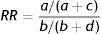
Relative risk (RR) to compare groups
- Risk of intervention group=A/(A+C)=0.697 or 69.7%
- Risk of comparison group=B/(B+D)=0.182 or 18.2%
- RR=(A/(A+C))/(B/(B+D))=0.697/0.182=3.83
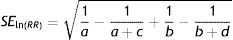
- Standard error for RR (SEln(RR)): Eq. (5.2)
• SEln(RR)=√((1/A)−(1/(A+C))+(1/B)−(1/(B+D)))=√((1/23)−(1/(33))+(1/6)−(1/(33)))=0.387
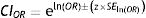
- 95% CIRR=eln(RR)±(z×SEln(RR))=e1.342865±(1.96×0.387)=e0.584345to2.101385=1.79 to 8.17
95% confidence interval (CI) for RR
The 95% frequentist CI around the RR found for pelvic floor muscle strength after eight weeks from baseline was 1.79 to 8.17 in the 6-point MOS. This means that we can be 95% confident that women with pelvic floor dysfunctions would present, on average, an RR between 1.79 and 8.17 when comparing the intervention with the comparison group, based on hypothesized repeats of the experiment. Since the 95% CI does not contain the null effect (i.e., one), which represents the null hypothesis (i.e., the same risk for both groups), we can conclude that this effect was statically significant, which means that we can be 95% confident that the intervention would be effective on increasing the risk of women changing the MOS for the better, which means strengthen the pelvic floor muscles, compared to the comparison group in repeats of the experiment.
Odds ratio (OR) to compare groups
- Odds of intervention group=(A/(A+C))/(C/(A+C))=A/C=2.30
- Odds of comparison group=(B/(B+D))/(D/(B+D))=B/D=0.2222…
- OR=(A/C)/(B/D) = 2.30/0.22=10.35
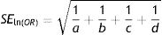
- SE ln(OR): Eq. (6.2)
• SEln(OR)=√((1/A)+(1/B)+(1/C)+(1/D))=√((1/23)+(1/6)+(1/10)+(1/27))=0.589
- 95% CIOR=eln(OR)±(z×SEln(OR))=e2.336987±(1.96×0.589)=e1.182547to3.491427=3.26 to 32.84
95% confidence interval (CI) for OR
The 95% frequentist CI around the OR found for pelvic floor muscle strength after eight weeks from baseline was 3.26 to 32.84 in the 6-point MOS. This means that we can be 95% confident that women with pelvic floor dysfunctions would present, on average, an OR between 3.26 and 32.84 when comparing the intervention with the comparison group, based on hypothesized repeats of the experiment. Since the 95% CI does not contain the null effect (i.e., one), which represents the null hypothesis (i.e., the same odds for both groups), we can conclude that this effect was statically significant, which means that we can be 95% confident that the intervention would be effective on increasing the odds of women changing the MOS for the better, which means strengthen the pelvic floor muscles, compared to the comparison group in repeats of the experiment.
The most known and widely used approach for statistical inference is the frequentist approach, also known as the classical (Neyman–Pearson) statistical approach.3,4 The frequentist approach for statistical inference is based on sampling distributions and the Central Limit Theorem (CLT).3,5 This explains the term “long-run frequency” attached to the interpretation of outcomes estimated using this approach (see the section “Interpreting frequentist 95% CIs”), and the term “frequentist” to refer to this statistical thinking. The frequentist approach treats the population parameters of interest as fixed values.2,3,6
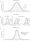
For example, let's assume a population distribution with mean (μ)=0 and SD (σ)=5 (Fig. 1A). In reality, we usually do not know the true mean and standard deviation in the population; however, for the sake of examples, we are defining the population distribution in Fig. 1A. Let us say a researcher has collected data from this population, and the sample mean (x¯1)=0.4 and the sample SD (s1)=4.8 (Fig. 1B, “Data collected”). The sample mean is considered the best guess of the sampling distribution mean (i.e., the mean of the sample means represented by Fig. 1C). In turn, the sampling distribution (Fig. 1C) is considered a long-run frequency of samples, including the one the researcher has collected data (sample 1 in Fig. 1B, “Data collected”), but also considering a set of hypothetical samples (samples 2–100 represented in Fig. 1B, “Hypothetical samples”) that do not exist (i.e., the researcher has not collected data for this hypothetical samples). This has some implications that are discussed in the section “Disadvantages of frequentist 95% CIs”.
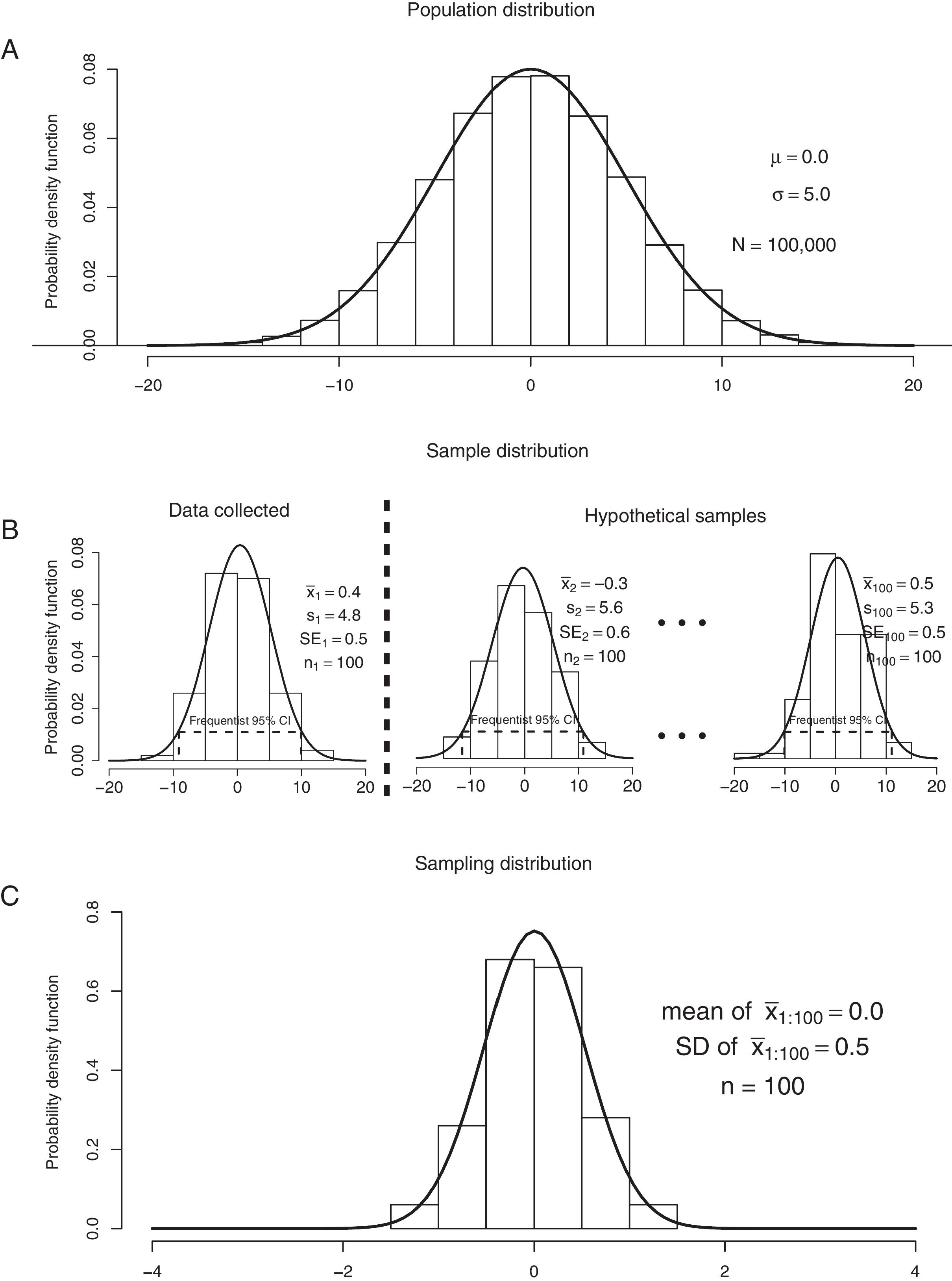
Graphical representation of: (A) a population distribution; (B) samples 1 to 100 from the population distribution (n=100 for each sample); and (C) the sampling distribution. “N”, population size. “n”, sample size. “μ”, population mean. “σ”, population standard deviation. “x¯”, sample mean. “s”, sample standard deviation. “SE”, standard error. “CI”, confidence interval.
There are several methods for estimating frequentist 95% CIs. In this masterclass we will describe the methods implemented in the Physiotherapy Evidence Database (PEDro) CI calculator, which can be downloaded in English at https://www.pedro.org.au/english/downloads/confidence-interval-calculator/.7 The reader can follow the estimations described in the case studies in Boxes 1 and 2 using the PEDro CI calculator.
Estimating frequentist CIsMeanEq. (1) describes CI formula for a mean (x¯). The critical value “t” is based on the t distribution attached with a particular probability level and degrees of freedom. For a 95% CI, the probability level must be set as 0.95 (or 95%) and the degrees of freedom are determined by subtracting 1 from the sample size (n−1). The SE of the sample mean can be estimated by Eq. (1.1).
Mean difference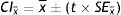

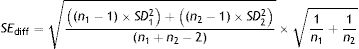
Eq. (2) describes the CI calculation for a mean difference (x¯1−x¯2). The critical value “t” is based on the t distribution attached with a particular probability level and degrees of freedom. For a 95% CI, the probability level must be set as 0.95 (or 95%) and the degrees of freedom are determined by subtracting 2 from the overall sample size (n1+n2−2). “SEdiff” refers to the SE of the difference between the two sample means assuming equal variances (Eq. (2.1)). Box 1 describes a case study using mean difference and its 95% CI.
Proportion and odds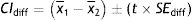
Eq. (3) describes the Wilson score method8,9 to estimate the CI for a proportion (p). The critical value “z” is based on the normal (Gaussian) distribution attached with a particular probability level. For a 95% CI, the critical value “z” is approximately 1.96. The odds and its 95% CI can be obtained by converting the proportions to odds using Eq. (3.1).
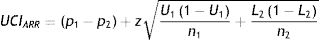
Absolute risk reduction (ARR)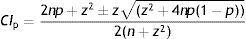

Eqs. (4.1) and (4.2) describe the Newcombe–Wilson method9,10 to estimate the lower (LCIARR) and upper (UCIARR) limits of the CI for the ARR, respectively. The letters “L” and “U” represents the lower and upper limits of the proportions for groups 1 and 2, which can be estimated using Equation 3.
Relative risk (RR) and odds ratio (OR)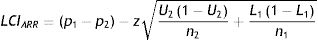
Eqs. (5) and (6) describe the CI calculation for the RR and for the OR, respectively.11 In Eqs. (5.1), (5.2), (6.1) and (6.2), “A” represents the number of individuals with the event in group 1; “B” represents the number of individuals with the event in group 2; “C” represents the number of individuals without the event in group 1; and “D” represents the number of individuals without the event in group 2. These values can be determined in a 2 by 2 table.11Box 2 describes a case study using RR, OR and their respective 95% CIs.
Interpreting frequentist CIs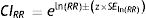

The frequentist CI has a long-run frequency interpretation, that is: random samples from the same target population and with the same sample size would yield CIs that contain the true (unknown) estimate in a frequency (percentage) set by the confidence level. However, we usually do not have several random samples from the same population; instead we collect data from only one sample of the population of interest and compute the CI for this particular sample. The interpretation of this particular CI would be: we can be XX% confident that the true (unknown) estimate would lie within the lower and upper limits of the CI, based on hypothesized repeats of the experiment.
For the 95% CI, this would imply that if we repeat an experiment 100 times and compute the 95% CI for all 100 experiments (Fig. 1B), then 95 (95%) of these CIs would contain the true (unknown) estimate, while 5 (5%) of these CIs would not contain the true (unknown) estimate. This true (unknown) estimate is represented in Fig. 1C by the mean of the sampling distribution (i.e., “mean of x¯1:100=0.0”), which frequentists use as a proxy for the population mean represented by Fig. 1A. But let us suppose we have collected data from only one sample of the target population (which is usually the case), that is represented by the sample “Data collected” in Fig. 1B. The 95% CI yielded from this particular sample can be interpret as follows: we can be 95% confident that the true (unknown) estimate would lie within the lower and upper limits of the CI, based on hypothesized repeats of the experiment.
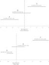
Regarding statistical significance, if the CI does not contain the null hypothesized value, this would indicate statistical significance for the particular significance level set by the investigator. For example, in case of a between-group mean difference in a randomized controlled trial, the null hypothesized value represented by the null hypothesis (H0) is zero (i.e., no difference between the groups: x¯1−x¯2=0). If the 95% CI does not contain zero and the limits are negative (e.g., −4.0 to −1.0; Fig. 2A) this means that we can be 95% confident that the true (unknown) between-group mean difference would, on average, lie within negative values, indicating that we can be 95% confident that the intervention group would present a lower mean compared to the comparison group. Moreover, if the 95% CI does not contain zero and the limits are positive (e.g., 0.5 to 3.5; Fig. 2C) this means that we can be 95% confident that the true (unknown) between-group mean difference would, on average, lie within positive values, indicating that we can be 95% confident that the intervention group would present a higher mean compared to the comparison group. Both scenarios would indicate a statistically significant result at a significance level of 0.05 (1–0.95) or 5%, since both CIs do not contain zero. These results would certainly yield a p-value lower than 0.05. However, if the 95% CI contains zero (e.g., −2.0 to 1.0; Fig. 2B) this means that we can be 95% confident that the true (unknown) between-group mean difference would, on average, lie within a negative and a positive value, indicating that we cannot be 95% confident that the intervention group would present a lower or a higher mean compared to the comparison group. This would indicate a non-statistically significant result, certainly yielding a p-value higher than 0.05 (for another example and interpretation, see Box 1).
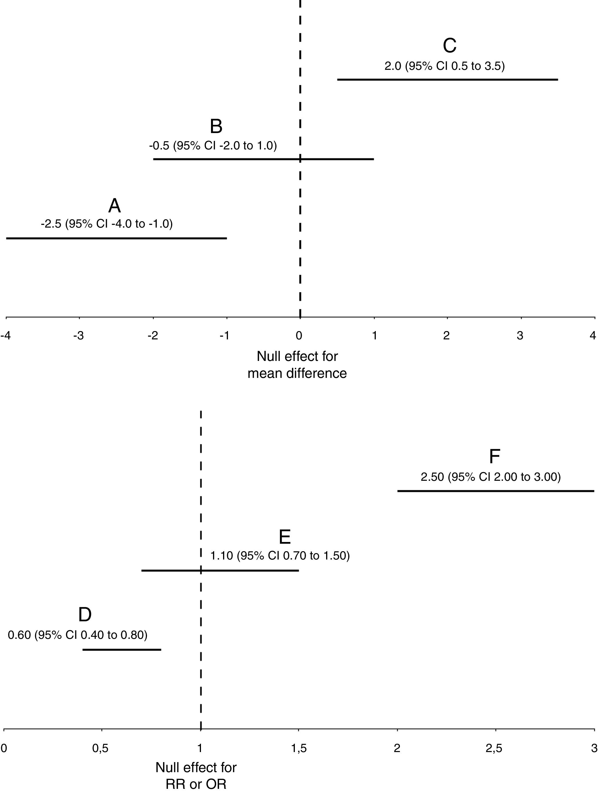
Graphical representation of statistically significant (A, C, D, and F) and non-statistically significant (B and E) results for frequentist 95% confidence intervals or Bayesian 95% credible intervals. For simplicity, both frequentist and Bayesian intervals are interchangeable in this figure, and they are represented with the acronym “CI”. “RR”, relative risk. “OR”, odds ratio.
In case of ratios, such as RR and OR, the null hypothesized value represented by the null hypothesis (H0) is 1 (i.e., same proportion or odds in both groups: p1/p2=1). If the 95% CI does not contain 1 and the limits are lower than 1 (e.g., 0.40 to 0.80; Fig. 2D) this means that we can be 95% confident that the true (unknown) ratio would, on average, lie within values lower than 1, indicating that we can be 95% confident that the intervention group would present a lower event proportion compared to the comparison group. Moreover, if the 95% CI does not contain 1 and the limits are higher than 1 (e.g., 2.0 to 3.0; Fig. 2F) this means that we can be 95% confident that the true (unknown) ratio would, on average, lie within values higher than 1, indicating that we can be 95% confident that the intervention group would present a higher event proportion compared to the comparison group. Both scenarios would indicate a statistically significant result at a significance level of 0.05 (1–0.95) or 5%, since both CIs do not contain 1. These results would certainly yield a p-value lower than 0.05. However, if the 95% CI contains 1 (e.g., 0.70 to 1.50; Fig. 2E) this means that we can be 95% confident that the true (unknown) ratio would, on average, lie within a value lower than 1 and a value higher than 1, indicating that we cannot be 95% confident that the intervention group would present a lower or a higher event proportion compared to the comparison group. This would indicate a non-statistically significant result, certainly yielding a p-value higher than 0.05 (for another example and interpretation, see Box 2). The same interpretation approach for RR can also be applied to OR. However, one should note that RR and OR are not the same measure (Box 2).
Advantages of using frequentist CIs rather than p-valuesThe frequentist approach is well known for performing hypothesis testing. Frequentist hypothesis testing lies in accepting or rejecting the null hypothesis (H0) by calculating the famous “p-value”. The p-value is defined as the probability of observing the acquired or a more extreme result in a hypothetical series of repeats of the experiment (i.e., sampling distribution), given that the null hypothesis is true.3,4 Health science researchers usually define a significance level of 0.05 (or 5%) for hypothesis testing. Therefore, one rejects the null hypothesis when a p-value is smaller than 0.05, which means that the probability of observing the actual or a more extreme estimate, given that the null hypothesis is true, is very low, supporting the conclusion that the null hypothesis might not be true. On the other hand, one accepts the null hypothesis when a p-value is equal to or greater than 0.05, which means that the probability of observing the actual or a more extreme estimate, given that the null hypothesis is true, is moderate to high, supporting the conclusion that the null hypothesis might be actually true. Another simple way of interpreting p-values is the following: the smaller the p-value the greater the evidence against the null hypothesis and, therefore, the results suggest that the alternative hypothesis (H1) might be more likely.
However, criticisms have been raised on how researchers and health professionals have been misinterpreting, misusing, and overemphasizing frequentist hypothesis testing, especially the p-value.4,12,13 These criticisms include the following3,4,12–14:
- •
The p-value is not the probability that the null hypothesis is (or is not) true, which would be formally represented as p(H0|y); “H0” represents the null hypothesis and “y” represents the observed data. However, many researchers and health professionals are tempted to interpret the p-value this way, leading to misinterpretations. Actually, the p-value is a measure of the extremeness of the actual result given the null hypothesis, which may be formally represented as p(y|H0). Perhaps due to non-familiarity with these concepts, the p-value interpretation most used in research and in practice is dichotomized, i.e., statistically significant or not statistically significant based on a threshold of 0.05. This may avoid the probability misinterpretation of p-values, but also oversimplifies the information provided by them.
- •
The dichotomized interpretation approach of p-values, which are widely used in research and in practice, allows for accepting or rejecting the null hypothesis without questioning the effect size or the variability (e.g., uncertainty or precision) of the effect estimate.
- •
The p-value seems to have a large sample-to-sample variability, indicating that this measure is probably not reliable on indicating the strength of evidence against the null hypothesis.
The frequentist CI has been suggested as an alternative to p-values.12,13 It has the advantage of describing the variability of the estimate and its width indicates the precision of the estimate.2 Therefore, researchers have recommended that effect estimates should be followed by their CIs (usually with a 95% confidence level) in scientific reportings.1,15 However, the current use of the frequentist CI has also raised some concerns, which would be discussed in the next section (i.e., “Disadvantages of using frequentist CIs”).
Disadvantages of using frequentist CIsWe believe that the use of the frequentist CI has two potential disadvantages. Firstly, the long-run frequency interpretation of the frequentist CI is not friendly. Therefore, many researchers and health professionals have misinterpreted the frequentist CI.15 For the 95% CI, a common misinterpretation is the following: there is a 95% probability that the true (unknown) effect estimate lies within the 95% CI. This interpretation is not accurate for the frequentist CI, since the frequentist approach treats the population parameter as a fixed (unknown) value and, therefore, this fixed value is either inside or outside the interval with 100% (or 0%) probability.2,6 Actually, the “probability interpretation” that clinicians usually use in clinical practice refers to the Bayesian interval (see the section “Bayesian approach for CIs”).3,15 Thereby, the accurate interpretation for the frequentist 95% CI would be the following: if we repeat an experiment over and over again (graphically represented by Fig. 1B) and we compute the 95% CI for all experiments, then 95% of these CIs would contain the true (unknown) estimate (represented by “mean of x¯1:100” in Fig. 1C), while 5% of these CIs would not contain the true (unknown) estimate (Boxes 1 and 2). A graphical representation of the frequentist 95% CI can be found in Fig. 1B.
Secondly, many researchers and health professionals oversimplify the interpretation of the frequentist 95% CI by dichotomizing it in statistically significant or non-statistically significant and, therefore, hampering a proper discussion on the values, the width (i.e., precision) and the practical implications of such interval. This would lead to some limitations and criticisms discussed earlier in this masterclass for the use of p-values, ruling out the advantages of using frequentist CIs rather than p-values. Therefore, there is no additional benefit in replacing the use of p-values by an oversimplified (i.e., dichotomized) interpretation of the frequentist CI.
Illustrative example of frequentist CIsA randomized controlled trial had investigated the effectiveness of back school versus McKenzie exercises in individuals with chronic nonspecific low back pain.16 The primary outcomes were pain intensity (0–10 pain numerical rating scale) and disability (Roland–Morris Disability Questionnaire analyzed as a 0–24 numeric scale) one month after randomization. The between-group difference (adjusted for within-group differences) for pain intensity was 0.66 with a 95% CI of −0.29 to 1.62, meaning that we can be 95% confident that the true (unknown) effect would lie between −0.29 and 1.62, based on hypothesized repeats of the experiment. For disability, the between-group difference (adjusted for within-group differences) was 2.37 in favor of McKenzie with a 95% CI of 0.76 to 3.99, meaning that we can be 95% confident that the true (unknown) effect would lie between this CI, based on hypothesized repeats of the experiment. The null hypothesized effect was zero (i.e., no difference between groups). The 95% CI for pain intensity contained the null effect (i.e., zero), meaning that the result was not statistically significant. For disability, the 95% CI did not contain the null effect, meaning that the result was statistically significant. Up to now, the conclusions would be the same if one had used the dichotomized interpretation of p-values instead of the dichotomized interpretation of CIs. However, despite significance, the effect for disability was considered small, because in this case, clinicians could expect that their clinical results for disability would fall approximately within 0.76 to 3.99 points on a 0–24 points measure. This interpretation would not be possible when considering only the p-value (which only measures the extremeness of the result under the null hypothesis) or the dichotomized interpretation of the CI. Therefore, the authors concluded that McKenzie exercise were not superior than back school for improving pain intensity in individuals with chronic nonspecific low back pain, and were only slightly more effective for disability.16
Bayesian approach for CIsBayesian inference is a statistical approach aiming at estimating a certain parameter (e.g., a mean or a proportion) from the population distribution, given the evidence provided by the observed (i.e., collected) data.3 Therefore, the Bayesian approach for statistical inference is considered a more direct or natural approach to answer a research question, since it estimates the parameter of interest directly from the population distribution (Fig. 1A) instead of estimating from the sampling distribution as the frequentist approach (Fig. 1C). The Bayesian approach treats the parameters of interest as random variables, and, therefore, parameters can be described with probability distributions.3,17 One of the main characteristic of the Bayesian approach is the compromise of prior evidence with the observed data. Prior evidence and the observed data are represented with probability distributions that, in Bayesian terminology, are defined as prior and likelihood distributions, respectively. The prior distribution is combined with the likelihood distribution in order to update the previous knowledge, resulting in the posterior distribution, which is formally represented as p(θ|y); “θ” represents the parameter of interest and “y” represents the observed data.3
The outcome of a Bayesian analysis is the posterior distribution. The posterior distribution can be summarized by measures of central tendency (e.g., median, mean or mode) and measures of uncertainty (e.g., variance or standard deviation). One of the most used measures of uncertainty in Bayesian inference is the Bayesian credible interval (CrI), which is analogous to the CI in the frequentist approach.
Estimating Bayesian CrIsDescribing and discussing the computation of posterior distributions are beyond the scope of this masterclass. However, once the posterior distribution that represents the updated knowledge about a parameter of interest is defined, obtaining the CrI is straightforward. There are typically two types of Bayesian CrIs: (1) equal tail interval; and (2) highest posterior density (HPD) interval. The following sections will be focused on defining, explaining and interpreting such intervals.
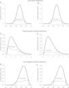
Equal tail CrIThe Bayesian equal tail CrI method returns threshold values of the posterior distribution that represent an interval with the probability of interest (e.g., 95%) of the distribution mass around the center of the distribution (Fig. 3A). In other words, the lower limit of the 95% equal tail CrI is the quantile representing a probability of 0.025 (or the 2.5% percentile) of the posterior distribution, while the upper limit of the equal tail CrI is the quantile representing a probability 0.975 (or the 97.5% percentile) of the posterior distribution. An advantage of estimating the equal tail Bayesian CrI is that this interval is easily calculated. However, a common concern related to the equal tail Bayesian CrI is that it might yield estimate values with lower probability inside the interval than outside the interval when the posterior distribution is not symmetric (i.e., right or left skewed).3 When this occurs, the meaning would be that some values would have a higher probability of representing the parameter when outside the interval compared to some values inside the interval. Graphically, this would yield a shift line connecting the lower and upper limits for this interval (Fig. 3C and E). Since this situation is not desired, another method has been proposed in order to estimate Bayesian CrIs: the HPD interval, which is discussed in the next section (i.e., “Highest posterior density (HPD) CrI”).
Highest posterior density (HPD) CrI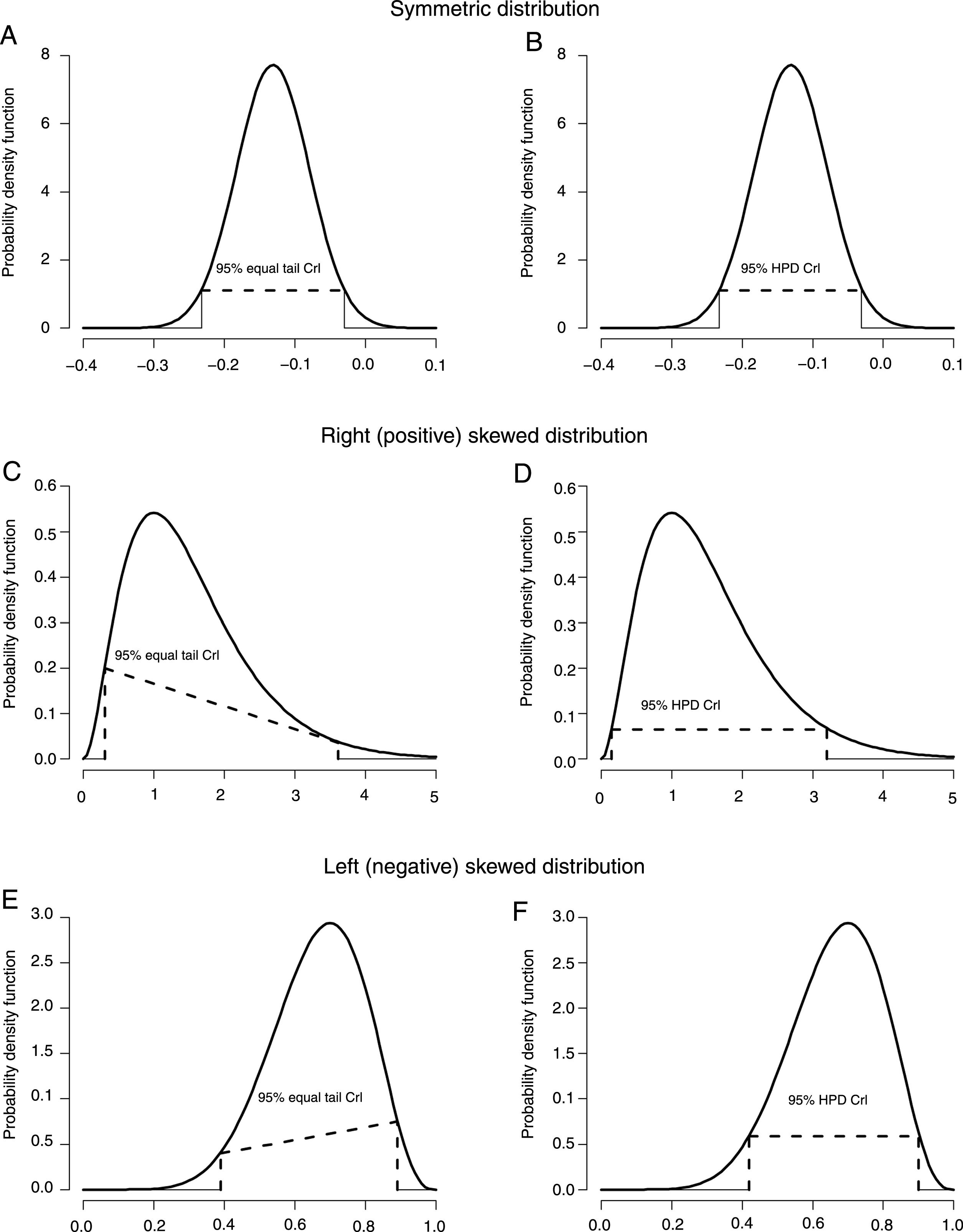
The Bayesian HPD CrI method returns threshold values of the posterior distribution that represent an interval with the probability of interest (e.g., 95%) of the distribution mass around the center of the distribution, holding true the assumption that all values inside the interval have higher probabilities of representing the parameter than all the values outside the interval. For example, for a 95% HPD CrI, the interval contains 95% of the mass of the posterior distribution around the center of the distribution, and all values inside the interval are more likely to represent the parameter than the values outside the interval. Graphically, this would always yield a straight line connecting the lower and upper limits for this interval (Fig. 3B, D and F). For symmetric posterior distributions, the HPD CrI is equivalent to the equal tail Bayesian CI (Fig. 3A and B).3 A disadvantage of the HPD CrI method is that the computation of the interval is more complex compared to the equal tail CrI method, since the HPD CrI estimation requires numerical optimization.3
Interpreting Bayesian CrIsBayesian CrIs have a more natural interpretation than frequentist CIs.3 This is due to the fact that the Bayesian CrI estimates the most likely values of the parameter of interest directly from the computed posterior distribution, which, in turn, represents all knowledge and evidence about the population distribution at the moment. The interpretation of the Bayesian 95% CrI is the following: there is a 95% probability that the true (unknown) effect estimate (represented by “μ” in Fig. 1A) would lie within the interval, given the evidence provided by the observed data.3,15
The way we judge if there is a statistical significance result when interpreting the Bayesian CrI is similar to the frequentist CI. However, one should note that the interpretation of the Bayesian CrI is rather different from the frequentist CI. For example, in case of a between-group mean difference, the null effect is zero (i.e., no difference between the groups: x¯1−x¯2=0). Let us suppose that a 95% CrI is composed of the following limits: −4.0 to −1.0 (Fig. 2A). This would indicate that there is a 95% probability that the population mean difference would lie between −4.0 and −1.0, given the observed data. In other words, the most plausible values (i.e., −4.0 to −1.0) with higher probability of representing the true (unknown) estimate indicate that the mean of the intervention group would be lower compared to the comparison group, with at least a 95% probability. Moreover, let us suppose that a 95% CrI is composed of the following limits: 0.5 to 3.5 (Fig. 2C). This would indicate that there is a 95% probability that the population mean difference would lie between 0.5 and 3.5, given the observed data. In other words, the most plausible values (i.e., 0.5 to 3.5) with higher probability of representing the true (unknown) estimate indicate that the mean of the intervention group would be higher compared to the comparison group, with at least a 95% probability. Both scenarios would indicate a statistically significant result at a significance level of 0.05 (1–0.95) or 5%, since both CrIs do not contain zero. However, in case of a 95% CrI composed of the following limits: −2.0 to 1.0 (Fig. 2B), this would indicate that there is a 95% probability that the population mean difference would lie between −2.0 and 1.0, given the observed data. Since the most plausible values (i.e., −2.0 to 1.0) with higher probability of representing the true (unknown) estimate indicate that the mean of the intervention group could be either lower or higher compared to the comparison group, this would indicate a non-statistically significant result.
In case of ratios, such as RR and OR, the null effect is 1 (i.e., same proportion or odds in both groups: p1/p2=1). Let us suppose that a 95% CrI for an RR is composed of the following limits: 0.40 to 0.80 (Fig. 2D). This would indicate that there is a 95% probability that the population RR would lie between 0.40 and 0.80, given the observed data. In other words, the most plausible values (i.e., 0.40 to 0.80) with higher probability of representing the true (unknown) estimate indicate that the event proportion of the intervention group would be lower compared to the comparison group, with at least a 95% probability. Moreover, let us suppose that a 95% CrI for an RR is composed of the following limits: 2.0 to 3.0 (Fig. 2F). This would indicate that there is a 95% probability that the population RR would lie between 2.0 and 3.0, given the observed data. In other words, the most plausible values (i.e., 2.0 to 3.0) with higher probability of representing the true (unknown) estimate indicate that the event proportion of the intervention group would be higher compared to the comparison group, with at least a 95% probability. Both scenarios would indicate a statistically significant result at a significance level of 0.05 (1–0.95) or 5%, since both CrIs do not contain 1. However, in case of a 95% CrI composed of the following limits: 0.70 to 1.50 (Fig. 2E), this would indicate that there is a 95% probability that the population RR would lie between 0.70 and 1.50, given the observed data. Since the most plausible values (i.e., 0.70 to 1.50) with higher probability of representing the true (unknown) estimate indicate that the event proportion of the intervention group could be either lower or higher compared to the comparison group, this would indicate a non-statistically significant result. The same interpretation approach of RR can also be applied to OR. However, one should note that RR and OR are not the same measure (Box 2).
Advantages of using Bayesian CrIsA clear advantage of Bayesian CrIs is the interpretability of such measures. For example, let us consider the frequentist 95% CI related to the effectiveness of back school compared to McKenzie exercises on disability discussed earlier in this masterclass (see the section “Illustrative example of frequentist CIs”), that is 0.76 to 3.99. As discussed earlier, the interpretation of this frequentist 95% CI is that, considering a hypothetical series of repeats of the experiment, we can be 95% confident that the true (unknown) effect estimate (represented by “mean of x¯1:100” in Fig. 1C) would lie between 0.76 and 3.99. Now, let us suppose that this interval was estimated using Bayesian inference. Considering the same interval as a Bayesian CrI, the interpretation would be that there is a 95% probability that the true (unknown) effect estimate (represented by “μ” in Fig. 1A) lies within 0.76 to 3.99, given the observed data. The Bayesian CrI is considered to be easier to interpret than the frequentist CI, because:
- •
The Bayesian CrI can be interpreted in a probabilistic way, which clinicians usually use in clinical practice even for frequentist CIs.3 This indicates the preference of clinicians for this probabilistic interpretation.
- •
The Bayesian approach reflects a direct estimate from the population distribution (Fig. 1A) represented by the actual computed posterior distribution, instead of estimating from the hypothetical sampling distribution (Fig. 1B and C) in the frequentist approach.
A clear disadvantage of using Bayesian CrIs is the complexity of computing posterior distributions, especially in complex problems/analyses conducted in, for example, randomized controlled trials. In the past, this imposed a very important barrier to the use of Bayesian inference. However, considering the recent advantages in computer science and technology, the use of Bayesian inference was significantly facilitated especially in complex situations. Therefore, computation issues should not preclude Bayesian analyses nowadays. However, knowledge and skills for performing such analyses are clearly remaining barriers that should be considered in biostatistics education for health scientists and for health professionals. This might generate work opportunities for clinicians, including physical therapists, as suggested by Casals and Finch.18,19
Illustrative example of Bayesian CrIsA 6-month randomized controlled trial had investigated the effectiveness of an online tailored advice package (i.e., TrailS6) compared to general advice on preventing running-related injuries (RRI) in trail runners.20 The main result was presented by an ARR of −13.1% (i.e., the intervention reduced the risk of sustaining RRIs in 13.1%), with a 95% HPD CrI of −23.3% to −3.1%. The interpretation of this 95% HPD CrI is that there was a 95% probability that the true (unknown) preventive effect would have been within −23.3% to −3.1%.20 In other words, the most plausible values (i.e., −23.3% to −3.1%) with higher probability of representing the true (unknown) estimate indicate that the intervention group would present a lower risk of RRIs compared to the comparison group, with at least a 95% probability. We believe that this interval is more natural an easy-to-interpret than the frequentist CI. The authors of the trial concluded that the online tailored advice package (TrailS6) was effective on preventing RRIs in trail runners.
ConclusionsWe believe that, as recommended by Freire et al.,1 the use and reporting of 95% CIs should be encouraged even when p-values are presented. Decision-making should neither be made considering only the dichotomized interpretation of p-values nor the dichotomized interpretation of CIs (i.e., statistically significant or non-statistically significant). Instead, a more in-depth analysis and interpretation of the values and width (i.e., precision) of CIs are recommended in order to avoid oversimplification of these rich measures. Frequentist CIs are alternative and preferable measures compared to p-values. However, the interpretability of the frequentist approach, which is based on hypothetical series of repeats of the experiment (i.e., sampling distribution) given that the null hypothesis is true, opens the opportunity for the use of Bayesian CrIs, that are more naturally and easily interpretable. Training and education may enhance knowledge and skills related to estimating, understanding and interpreting uncertainty measures, reducing the barriers for their use under either frequentist or Bayesian approaches.
FundingThis masterclass had no funding source of any nature.
Conflicts of interestThe authors declare no conflicts of interest.
Luiz Hespanhol was granted with a Young Investigator Grant from the São Paulo Research Foundation (FAPESP), grant 2016/09220-1. Caio Sain Vallio was granted with a PhD scholarship from FAPESP, process number 2017/11665-4. Bruno T Saragiotto was granted with a Young Investigator Grant from FAPESP, grant 2016/24217-7.


